Get Started
Contrails.org API is a RESTful API that provides contrail modeling and mitigation tools.
This notebook shows basic usage of Contrails.org API from a Python notebook using the requests package to send HTTP requests.
You can interact with Contrails.org API with any HTTP compatible client (i.e. curl, Postman).
Authorization
Your API key must be provided in
x-api-keyrequest header.In this notebook, we pluck it from a preset environment variable.
Similarly, we parametrize the URL endpoint as an environment variable. The API base url is
https://api.contrails.org.Contact api@contrails.org to request a user account.
[1]:
import os
from pprint import pprint
[2]:
URL = "https://api.contrails.org"
API_KEY = os.environ["CONTRAILS_API_KEY"]
HEADERS = {"x-api-key": API_KEY}
Research API (/v0)
The Research API (/v0/trajectory, v0/grid) provides hosted versions of pycontrails models run with re-analysis and forecast meteorology provided by ECMWF.
See the Research API /v0 notebook for details on calculating model outputs on flight trajectories and meteorology grids.
[3]:
import matplotlib.pyplot as plt  # pip install matplotlib
import numpy as np  # pip install numpy
import pandas as pd  # pip install pandas
[4]:
n_waypoints = 100
t0 = "2022-06-07T00:15:00"
t1 = "2022-06-07T02:30:00"

flight = {
    "longitude": np.linspace(-29, -50, n_waypoints).tolist(),
    "latitude": np.linspace(45, 42, n_waypoints).tolist(),
    "altitude": np.linspace(33000, 38000, n_waypoints).tolist(),
    "time": pd.date_range(t0, t1, periods=n_waypoints).astype(str).tolist(),
    "engine_efficiency": np.random.default_rng(42).uniform(0.2, 0.4, n_waypoints).tolist(),
    "aircraft_mass": np.linspace(65000, 62000, n_waypoints).tolist(),
    "aircraft_type": "A320",
}
[5]:
import requests

r = requests.post(f"{URL}/v0/trajectory/sac", json=flight, headers=HEADERS)
print(f"HTTP Response Code: {r.status_code} {r.reason}\n")

r_json = r.json()
for k, v in r_json.items():
    print(f"{k}: {v}")
HTTP Response Code: 200 OK
flight_id: 1732208899718050
met_source_provider: ECMWF
met_source_dataset: ERA5
met_source_product: reanalysis
pycontrails_version: 0.52.1
humidity_scaling_name: histogram_matching
humidity_scaling_formula: era5_quantiles -> iagos_quantiles
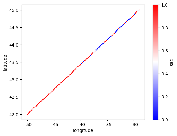
sac: [1.0, 0.0, 1.0, 1.0, 0.0, 1.0, 1.0, 1.0, 0.0, 0.0, 0.0, 1.0, 0.0, 1.0, 0.0, 0.0, 0.0, 0.0, 1.0, 0.0, 0.0, 0.0, 1.0, 1.0, 1.0, 0.0, 0.0, 0.0, 0.0, 1.0, 1.0, 1.0, 0.0, 0.0, 0.0, 0.0, 0.0, 0.0, 0.0, 1.0, 0.0, 1.0, 1.0, 0.0, 1.0, 1.0, 1.0, 1.0, 1.0, 0.0, 1.0, 0.0, 1.0, 1.0, 1.0, 1.0, 1.0, 1.0, 1.0, 1.0, 1.0, 1.0, 1.0, 1.0, 1.0, 1.0, 1.0, 1.0, 1.0, 1.0, 1.0, 1.0, 1.0, 1.0, 1.0, 1.0, 1.0, 1.0, 1.0, 1.0, 1.0, 1.0, 1.0, 1.0, 1.0, 1.0, 1.0, 1.0, 1.0, 1.0, 1.0, 1.0, 1.0, 1.0, 1.0, 1.0, 1.0, 1.0, 1.0, 1.0]
[6]:
flight_df = pd.DataFrame(flight).assign(sac=r_json["sac"])
flight_df.plot.scatter(x="longitude", y="latitude", c="sac", cmap="bwr", s=3);
[7]:
r = requests.post(f"{URL}/v0/trajectory/issr", json=flight, headers=HEADERS)
print(f"HTTP Response Code: {r.status_code} {r.reason}\n")

r_json = r.json()
for k, v in r_json.items():
    print(f"{k}: {v}")
HTTP Response Code: 200 OK
flight_id: 1732208904445308
met_source_provider: ECMWF
met_source_dataset: ERA5
met_source_product: reanalysis
pycontrails_version: 0.52.1
humidity_scaling_name: histogram_matching
humidity_scaling_formula: era5_quantiles -> iagos_quantiles
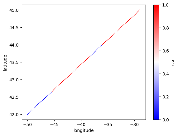
issr: [1.0, 1.0, 1.0, 1.0, 1.0, 1.0, 1.0, 1.0, 1.0, 1.0, 1.0, 1.0, 1.0, 1.0, 1.0, 1.0, 1.0, 1.0, 1.0, 1.0, 1.0, 1.0, 1.0, 1.0, 1.0, 1.0, 1.0, 1.0, 1.0, 1.0, 1.0, 1.0, 1.0, 1.0, 0.0, 0.0, 0.0, 0.0, 0.0, 0.0, 0.0, 0.0, 0.0, 0.0, 1.0, 1.0, 1.0, 1.0, 1.0, 1.0, 1.0, 1.0, 1.0, 1.0, 1.0, 1.0, 1.0, 1.0, 1.0, 1.0, 1.0, 1.0, 1.0, 1.0, 1.0, 1.0, 1.0, 1.0, 1.0, 1.0, 1.0, 1.0, 1.0, 1.0, 1.0, 1.0, 1.0, 1.0, 0.0, 0.0, 0.0, 0.0, 0.0, 0.0, 0.0, 0.0, 0.0, 0.0, 0.0, 0.0, 0.0, 0.0, 0.0, 0.0, 0.0, 0.0, 0.0, 0.0, 0.0, 0.0]
[8]:
flight_df["issr"] = r_json["issr"]
flight_df.plot.scatter(x="longitude", y="latitude", c="issr", cmap="bwr", s=1);
[9]:
r = requests.post(f"{URL}/v0/trajectory/cocip", json=flight, headers=HEADERS)
print(f"HTTP Response Code: {r.status_code} {r.reason}\n")
r_json = r.json()

# The /trajectory/cocip endpoint includes many fields in the response.
for k, v in r_json.items():
    v = str(v)
    if len(v) > 80:
        v = v[:77] + "..."
    print(f"{k}: {v}")
HTTP Response Code: 200 OK

cocip_max_contrail_age: 12 hours
cocip_dt_integration: 10 minutes
flight_id: 1732208906070747
met_source_provider: ECMWF
met_source_dataset: ERA5
met_source_product: reanalysis
pycontrails_version: 0.52.1
nvpm_data_source: ICAO EDB
engine_uid: 01P08CM105
humidity_scaling_name: histogram_matching
humidity_scaling_formula: era5_quantiles -> iagos_quantiles
sac: [1.0, 0.0, 1.0, 1.0, 0.0, 1.0, 1.0, 1.0, 0.0, 0.0, 0.0, 1.0, 0.0, 1.0, 0.0, 0...
nox_ei: [0.0076, 0.0076, 0.0076, 0.0076, 0.0076, 0.0076, 0.0076, 0.0076, 0.0076, 0.00...
nvpm_ei_n: [647000000000000.0, 647000000000000.0, 648000000000000.0, 649000000000000.0, ...
energy_forcing: [0.0, 0.0, 680000000000.0, 0.0, 0.0, 790000000000.0, 540000000000.0, 0.0, 0.0...
contrail_age: [0.0, 0.0, 112.0, 0.0, 0.0, 128.0, 127.0, 0.0, 0.0, 0.0, 0.0, 0.0, 0.0, 0.0, ...
initially_persistent: [1.0, 0.0, 1.0, 1.0, 0.0, 1.0, 1.0, 1.0, 0.0, 0.0, 0.0, 1.0, 0.0, 1.0, 0.0, 0...
[10]:
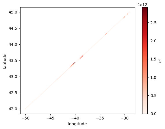
# Energy forcing is the primary model output.
ef = np.array(r_json["energy_forcing"], dtype=float)
ef
[10]:
array([0.00e+00, 0.00e+00, 6.80e+11, 0.00e+00, 0.00e+00, 7.90e+11,
       5.40e+11, 0.00e+00, 0.00e+00, 0.00e+00, 0.00e+00, 0.00e+00,
       0.00e+00, 0.00e+00, 0.00e+00, 0.00e+00, 0.00e+00, 0.00e+00,
       0.00e+00, 0.00e+00, 0.00e+00, 0.00e+00, 6.10e+11, 5.40e+11,
       0.00e+00, 0.00e+00, 0.00e+00, 0.00e+00, 0.00e+00, 0.00e+00,
       0.00e+00, 0.00e+00, 0.00e+00, 0.00e+00, 0.00e+00, 0.00e+00,
       0.00e+00, 0.00e+00, 0.00e+00, 0.00e+00, 0.00e+00, 0.00e+00,
       0.00e+00, 0.00e+00, 2.90e+11, 1.74e+12, 1.32e+12, 1.68e+12,
       0.00e+00, 0.00e+00, 0.00e+00, 0.00e+00, 2.92e+12, 2.54e+12,
       1.51e+12, 1.03e+12, 6.30e+11, 1.90e+11, 8.00e+10, 5.00e+10,
       5.00e+10, 6.00e+10, 6.00e+10, 7.00e+10, 1.20e+11, 1.50e+11,
       1.90e+11, 2.10e+11, 1.90e+11, 1.40e+11, 9.00e+10, 6.00e+10,
       2.00e+10, 0.00e+00, 0.00e+00, 0.00e+00, 0.00e+00, 0.00e+00,
       0.00e+00, 0.00e+00, 0.00e+00, 0.00e+00, 0.00e+00, 0.00e+00,
       0.00e+00, 0.00e+00, 0.00e+00, 0.00e+00, 0.00e+00, 0.00e+00,
       0.00e+00, 0.00e+00, 0.00e+00, 0.00e+00, 0.00e+00, 0.00e+00,
       0.00e+00, 0.00e+00, 0.00e+00, 0.00e+00])
[11]:
flight_df["ef"] = ef
flight_df.plot.scatter(x="longitude", y="latitude", c="ef", cmap="Reds", s=3);
[12]:
r = requests.post(f"{URL}/v0/trajectory/emissions", json=flight, headers=HEADERS)
print(f"HTTP Response Code: {r.status_code} {r.reason}\n")

r_json = r.json()
for k, v in r_json.items():
    v = str(v)
    if len(v) > 80:
        v = v[:77] + "..."
    print(f"{k}: {v}")
HTTP Response Code: 200 OK

flight_id: 1732208928844505
met_source_provider: ECMWF
met_source_dataset: ERA5
met_source_product: reanalysis
pycontrails_version: 0.52.1
nvpm_data_source: ICAO EDB
engine_uid: 01P08CM105
humidity_scaling_name: histogram_matching
humidity_scaling_formula: era5_quantiles -> iagos_quantiles
nox_ei: [0.0076, 0.0076, 0.0076, 0.0076, 0.0076, 0.0076, 0.0076, 0.0076, 0.0076, 0.00...
nvpm_ei_n: [647000000000000.0, 647000000000000.0, 648000000000000.0, 649000000000000.0, ...
[13]:
time = pd.to_datetime(flight["time"])

fig, ax = plt.subplots(figsize=(8, 4))
ax.plot(time, r_json["nox_ei"], label="nox_ei")

ax2 = ax.twinx()
ax2.plot(time, r_json["nvpm_ei_n"], color="orange", label="nvpm_ei_n")

lines1, labels1 = ax.get_legend_handles_labels()
lines2, labels2 = ax2.get_legend_handles_labels()
ax.legend(lines1 + lines2, labels1 + labels2, loc=0)

ax.set_ylabel("NOx emissions index")
ax2.set_ylabel("Nonvolatile particulate matter emissions index number")
ax.set_title("Emissions index for NOx and Nonvolatile Particulate Matter");

Data Availability
Grid endpoints in Contrails.org API serve data with varying availability. The /v0/grid/availability endpoint gives a range of times for which each /grid endpoint serves data.
[14]:
r = requests.get(f"{URL}/v0/grid/availability", headers=HEADERS)

print(f"HTTP Response Code: {r.status_code} {r.reason}")
pprint(r.json())
HTTP Response Code: 200 OK
{'cocip': ['2022-01-01T00:00:00Z', '2024-11-22T17:00:00Z'],
 'issr': ['2018-01-01T00:00:00Z', '2024-11-24T06:00:00Z'],
 'pcr': ['2018-01-01T00:00:00Z', '2024-11-24T06:00:00Z'],
 'sac': ['2018-01-01T00:00:00Z', '2024-11-24T06:00:00Z']}
SAC, ISSR, PCR
GET /v0/grid/sac
GET /v0/grid/issr
GET /v0/grid/pcr
The SAC, ISSR, and PCR grid endpoints all use similar conventions.
We demonstrate the SAC grid endpoint here. This endpoint accepts an optional engine_efficiency parameter that takes a default value of 0.3.
[15]:
import xarray as xr # pip install xarray
[16]:
time = "2022-06-07T02"
bbox = "-50,0,50,50"
params = {"time": time, "bbox": bbox, "engine_efficiency": 0.32}
r = requests.get(f"{URL}/v0/grid/sac", headers=HEADERS, params=params)
print(f"HTTP Response Code: {r.status_code} {r.reason}")
print(f"Response content-type: {r.headers['content-type']}")
HTTP Response Code: 200 OK
Response content-type: application/netcdf
netCDF Response Format
The default response format is netCDF. For the SAC endpoint, the 4D grid holds a single sac variable. The response can be written out and read with xarray.
[17]:
with open("sac.nc", "wb") as f:
    f.write(r.content)

da = xr.open_dataarray("sac.nc", engine="netcdf4")  # pip install netCDF4
da.coords  # each netCDF served in the API is a 4D grid
[17]:
Coordinates:
  * time          (time) datetime64[ns] 8B 2022-06-07T02:00:00
  * flight_level  (flight_level) int32 72B 270 280 290 300 ... 410 420 430 440
  * longitude     (longitude) float32 2kB -50.0 -49.75 -49.5 ... 49.5 49.75 50.0
  * latitude      (latitude) float32 804B 0.0 0.25 0.5 0.75 ... 49.5 49.75 50.0
[18]:
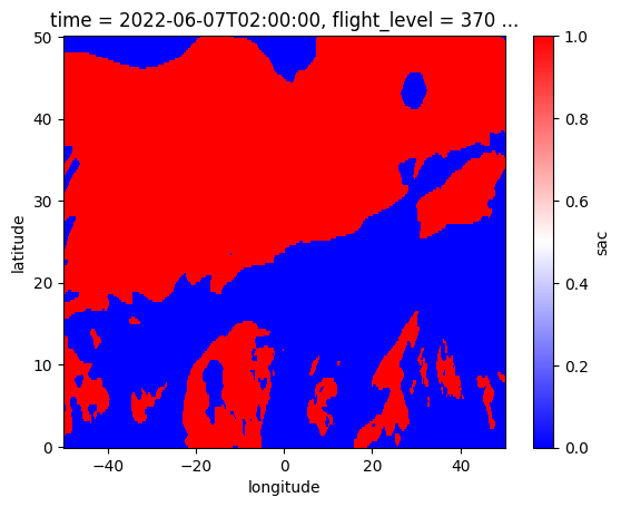
# The grid contains 18 flight levels ranging from 270 to 440.
da.flight_level.values
[18]:
array([270, 280, 290, 300, 310, 320, 330, 340, 350, 360, 370, 380, 390,
       400, 410, 420, 430, 440], dtype=int32)
[19]:
# We "squeeze" on time and select a single flight level to plot.
da.squeeze("time").isel(flight_level=10).plot(x="longitude", y="latitude", cmap="bwr");
GeoJSON Response Format
Contrails.org API supports two types of polygon formats: GeoJSON and KML.
We demonstrate the same grid endpoint using the GeoJSON representation here.
See the polygon documentation for additional examples including custom polygon simplification.
[20]:
params["format"] = "geojson"
r = requests.get(f"{URL}/v0/grid/sac", headers=HEADERS, params=params)

print(f"HTTP Response Code: {r.status_code} {r.reason}")
print(f"Response content-type: {r.headers['content-type']}")

r_json = r.json()
HTTP Response Code: 200 OK
Response content-type: application/json
[21]:
import shapely.geometry as sgeom # pip install shapely
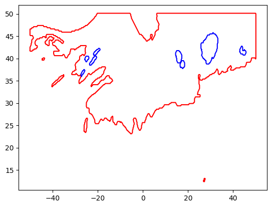
[22]:
# The response body is a GeoJSON FeatureCollection. Each feature contains polygons for each flight level.
print(f"GeoJSON type: {r_json['type']}")

# Extract a feature
feature = r_json["features"][8]
pprint(feature["properties"])  # print out the metadata

# Visualize with shapely
# Polygons can have both exterior and interior rings
polygons = sgeom.shape(feature["geometry"])
for poly in polygons.geoms:
    plt.plot(*poly.exterior.xy, color="red")  # color exterior red
    for interior in poly.interiors:
        plt.plot(*interior.xy, color="blue")  # and interior blue
GeoJSON type: FeatureCollection
{'description': 'Schmidt-Appleman contrail formation criteria',
 'engine_efficiency': 0.32,
 'humidity_scaling_formula': 'era5_quantiles -> iagos_quantiles',
 'humidity_scaling_name': 'histogram_matching',
 'level': 350,
 'level_long_name': 'Flight Level',
 'level_standard_name': 'FL',
 'level_units': 'hectofeet',
 'met_source_dataset': 'ERA5',
 'met_source_product': 'reanalysis',
 'met_source_provider': 'ECMWF',
 'name': 'sac',
 'polygon_iso_value': 0.5,
 'pycontrails_version': '0.52.1',
 'time': '2022-06-07T02:00:00Z'}

CoCiP
The
v0/grid/cocipendpoint is designed for research purposes. Please use the /v1 Contrail Forecast API to design production use cases (e.g. trials, flight planning, air traffic management) moving forward.
GET /v0/grid/cocip
The gridded CoCiP model (Engberg et al 2024) is an abstraction of the original CoCiP model . Instead of working with a single flight trajectory, the gridded version starts with a 4D vector field of trajectory segments each assumed to be in a nominal cruising state. The gridded model then evolves the segments over time using the same rules as the classical model.
Given a fixed trajectory, the original CoCiP model gives a precise prediction of contrail climate forcing resulting from that trajectory. Consequently, the /v0/trajectory/cocip endpoint should be favored when evaluating contrail forcing of a single flight. On the other hand, the gridded CoCiP model can be used to optimize an unknown trajectory over a 4D grid. The two models widely agree when a flight is in a nominal cruising state.
The /v0/grid/cocip endpoints requires an aircraft_type query parameter for CoCiP initialization.
Unlike all other endpoints, the model underpinning the /v0/grid/cocip endpoint has been precomputed. Only a limited set of 11 aircraft types are currently available.
A320
A20N
A321
A319
A21N
A333
A350
B737
B738
B789
B77W
netCDF Response Format
[23]:
params["aircraft_type"] = "A320"
params["format"] = "netcdf"

r = requests.get(f"{URL}/v0/grid/cocip", params=params, headers=HEADERS)
print(f"HTTP Response Code: {r.status_code} {r.reason}")
print(f"Content type: {r.headers['content-type']}")
HTTP Response Code: 200 OK
Content type: application/netcdf
[24]:
with open("cocipgrid.nc", "wb") as f:
    f.write(r.content)

ds = xr.open_dataset("cocipgrid.nc", engine="netcdf4")
ds.data_vars  # The CoCiP data comes with both energy forcing and contrail age
[24]:
Data variables:
    ef_per_m      (longitude, latitude, flight_level, time) float32 6MB ...
    contrail_age  (longitude, latitude, flight_level, time) timedelta64[ns] 12MB ...
[25]:
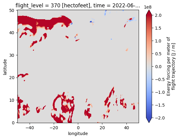
# The energy forcing variable is the primary model output.
da = ds["ef_per_m"]

# Print some metadata present in the netCDF
pprint(ds.attrs | da.attrs)

# We "squeeze" on time and select a single flight level to plot.
da.squeeze("time").isel(flight_level=10).plot(
    x="longitude", y="latitude", vmin=-2e8, vmax=2e8, cmap="coolwarm"
);
{'aircraft_type': 'A320',
 'cocip_dt_integration': '5 minutes',
 'cocip_max_contrail_age': '12 hours',
 'humidity_scaling_formula': 'rhi -> (rhi / rhi_adj) ^ rhi_boost_exponent',
 'humidity_scaling_name': 'exponential_boost_latitude_customization',
 'long_name': 'Energy forcing per meter of flight trajectory',
 'met_source_dataset': 'ERA5',
 'met_source_product': 'reanalysis',
 'met_source_provider': 'ECMWF',
 'name': 'cocip',
 'pycontrails_version': '0.32.2',
 'units': 'J / m'}
GeoJSON Response Format
We can specify an energy forcing threshold parameter when calling the endpoint. The response contains just polygons surrounding grid cells at which the ef_per_m exceeds the threshold.
In converting from the grid representation to the polygon representation, we exclude degenerate polygons and polygons whose area is doesn’t exceeds some minimal threshold. Excluding these edge cases allows us to focus on regions of high impact. See the polygon documentation for additional polygon simplification examples.
[26]:
params["format"] = "geojson"
params["threshold"] = 2e8
r = requests.get(f"{URL}/v0/grid/cocip", headers=HEADERS, params=params)

print(f"HTTP Response Code: {r.status_code} {r.reason}")
print(f"Response content-type: {r.headers['content-type']}")
r_json = r.json()
HTTP Response Code: 200 OK
Response content-type: application/json
[27]:
# Extract a feature
feature = r_json["features"][10]
pprint(feature["properties"])  # print out the metadata

# Visualize. We see polygons around regions of dark red in the previous plot.
polygons = sgeom.shape(feature["geometry"])
for poly in polygons.geoms:
    plt.plot(*poly.exterior.xy, color="red")  # color exterior red
    for interior in poly.interiors:
        plt.plot(*interior.xy, color="blue")  # and interior blue
{'aircraft_type': 'A320',
 'cocip_dt_integration': '5 minutes',
 'cocip_max_contrail_age': '12 hours',
 'humidity_scaling_formula': 'rhi -> (rhi / rhi_adj) ^ rhi_boost_exponent',
 'humidity_scaling_name': 'exponential_boost_latitude_customization',
 'level': 370,
 'level_long_name': 'Flight Level',
 'level_standard_name': 'FL',
 'level_units': 'hectofeet',
 'long_name': 'Energy forcing per meter of flight trajectory',
 'met_source_dataset': 'ERA5',
 'met_source_product': 'reanalysis',
 'met_source_provider': 'ECMWF',
 'name': 'ef_per_m',
 'polygon_iso_value': 200000000.0,
 'pycontrails_version': '0.32.2',
 'time': '2022-06-07T02:00:00Z',
 'units': 'J / m'}
Cleanup
[28]:
os.remove("sac.nc")
os.remove("cocipgrid.nc")
[4]:
import matplotlib.pyplot as plt  # pip install matplotlib
import numpy as np  # pip install numpy
import pandas as pd  # pip install pandas
[5]:
# create an example flight input
n_waypoints = 100
t0 = "2022-06-07T00:15:00"
t1 = "2022-06-07T02:30:00"

flight = {
    "longitude": np.linspace(-29, -50, n_waypoints).tolist(),
    "latitude": np.linspace(45, 42, n_waypoints).tolist(),
    "altitude": np.linspace(33000, 38000, n_waypoints).tolist(),
    "time": pd.date_range(t0, t1, periods=n_waypoints).astype(str).tolist(),
    "engine_efficiency": np.random.default_rng(42).uniform(0.2, 0.4, n_waypoints).tolist(),
    "aircraft_mass": np.linspace(65000, 62000, n_waypoints).tolist(),
    "aircraft_type": "A320",
}
[12]:
import requests  # pip install requests

# calculate the Schmidt-Appleman Criterion along the flight trajectory
r = requests.post(f"{URL}/v0/trajectory/sac", json=flight, headers=HEADERS)
print(f"HTTP Response Code: {r.status_code} {r.reason}\n")

# print out response
r_json = r.json()
for key, value in r_json.items():
    print(f"{key}: {value}")
HTTP Response Code: 200 OK

flight_id: 1738963287010274
met_source_provider: ECMWF
met_source_dataset: ERA5
met_source_product: reanalysis
pycontrails_version: 0.54.5
humidity_scaling_name: histogram_matching
humidity_scaling_formula: era5_quantiles -> iagos_quantiles
sac: [0.0, 0.0, 0.0, 0.0, 0.0, 1.0, 0.0, 0.0, 0.0, 0.0, 0.0, 1.0, 0.0, 1.0, 0.0, 0.0, 0.0, 0.0, 1.0, 0.0, 1.0, 0.0, 1.0, 1.0, 0.0, 0.0, 0.0, 0.0, 0.0, 1.0, 1.0, 1.0, 0.0, 0.0, 0.0, 0.0, 0.0, 0.0, 0.0, 0.0, 0.0, 1.0, 1.0, 0.0, 1.0, 1.0, 0.0, 0.0, 1.0, 0.0, 1.0, 0.0, 1.0, 1.0, 1.0, 1.0, 1.0, 1.0, 1.0, 1.0, 1.0, 1.0, 1.0, 1.0, 1.0, 1.0, 1.0, 1.0, 1.0, 1.0, 1.0, 1.0, 1.0, 1.0, 1.0, 1.0, 1.0, 1.0, 1.0, 1.0, 1.0, 1.0, 1.0, 1.0, 1.0, 1.0, 1.0, 1.0, 1.0, 1.0, 1.0, 1.0, 1.0, 1.0, 1.0, 1.0, 1.0, 1.0, 1.0, 1.0]
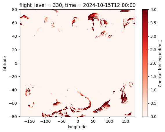
Forecast APIs
The Contrail Forecast APIs (/v1/grids, /v1/regions) implements a working specification for contrail forecast data designed for air traffic planners and managers implementing navigational contrail avoidance systems.
The data served from this endpoint contains contrail forcing scaled to a categorical index [0 - 4], with 0 representing no contrail harm and 4 representing the most harmful contrail forming regions.
See the Contrail Forecast /v1 notebook for details on accessing forecast data in netCDF and GeoJSON formats.
[16]:
import xarray as xr # pip install xarray
[17]:
# fetch netCDF forecast
params = {
    "time": "2024-10-15T12",  # format ISO 8601 (UTC)
    "aircraft_class": "default",
    "flight_level": 330,
}

resp = requests.get(f"{URL}/v1/grids", params=params, headers=HEADERS)
print(f"HTTP Response Code: {resp.status_code} {resp.reason}\n")

# Save request to disk, then open with xarray
with open("forecast.nc", "wb") as f:
    f.write(resp.content)

ds = xr.open_dataset("forecast.nc", engine="netcdf4")  # pip install netCDF4
HTTP Response Code: 200 OK
[18]:
# Plot lat x lon slice for this time x flight level
ds["contrails"].squeeze().plot(x="longitude", y="latitude", cmap="Reds");
ADS-B APIs
The ADS-B APIs (v1/adsb/) enables authorized users to access common ADS-B telemetry for contrails research purposes.
The underlying ADS-B data is provided by Spire Aviation.
See the Contrails ADS-B Access notebook for details on searching and downloading ADS-B data.
[ ]:
import matplotlib.pyplot as plt  # pip install matplotlib
import pandas as pd  # pip install pandas
import requests  # pip install requests
[ ]:
params = {
    "date": "2025-01-24T02"  # ISO 8601 (UTC)
}

r = requests.get(f"{URL}/v1/adsb/telemetry", params=params, headers=HEADERS)
print(f"HTTP Response Code: {r.status_code} {r.reason}\n")

# write out response content as parquet file
with open(f"{params['date']}.pq", "wb") as f:
    f.write(r.content)
[ ]:
# read parquet file with pandas
df = pd.read_parquet(f"{params['date']}.pq")

print("Number of unique flights:", df["flight_id"].nunique())
print("Number of unique waypoints:", len(df["flight_id"]))

df.head()