Polygon Simplification

This guide demonstrates customizing polygon requests to simplify the geometry of the returned polygons.

Contrails API supports both GeoJSON and KML polygon formats. We only work with GeoJSON polygons in this notebook.

This notebook uses Shapely to interact with polygons. In particular, GEOS is required to convert GeoJSON to Shapely polygons.

import json
import os
from pprint import pprint

import matplotlib.lines as mlines
import matplotlib.pyplot as plt
import pandas as pd
import requests
import shapely

# Define credentials
URL = "https://api.contrails.org"
api_key = os.environ["CONTRAILS_API_KEY"]
headers = {"x-api-key": api_key}

Query parameters

The following query parameters are used in the /v0/grid/issr endpoint:

• time: The time for the polygon prediction. Must be an ISO 8601 datetime string or unix timestamp (seconds since epoch).

• format: Set format=geojson to return polygons in GeoJSON format.

• interiors: Set interiors=true to return interior polygons.

• simplify: Used to control the extent to which polygon geometry is simplified.

• convex_hull: Set convex_hull=true to return the convex hull of the polygon.

• bbox: Used to downselect horizontally.

• flight_level: Used to downselect vertically.

Default parameters

Here, we request ISSR polygons at a single flight level using the default polygon simplify parameters.

params = {
    "time": "2023-02-10",
    "format": "geojson",
    "flight_level": 360,
}

r = requests.get(f"{URL}/v0/grid/issr", params=params, headers=headers)
print(f"HTTP Response Code: {r.status_code} {r.reason}")

HTTP Response Code: 200 OK

geojson = r.json()
feature = geojson["features"][0]

# Print out the metadata
pprint(feature["properties"])

# Convert the output to shapely
# Unfortunately, GEOS can't handle the altitude coordinate returned by the API
# Manually loop through and remove it
for coords in feature["geometry"]["coordinates"]:
    for poly in coords:
        for point in poly:
            del point[2]

multipoly = shapely.from_geojson(json.dumps(feature))

{'description': 'Ice super-saturated regions',
 'humidity_scaling_formula': 'era5_quantiles -> iagos_quantiles',
 'humidity_scaling_name': 'histogram_matching',
 'level': 360,
 'level_long_name': 'Flight Level',
 'level_standard_name': 'FL',
 'level_units': 'hectofeet',
 'met_source_dataset': 'ERA5',
 'met_source_product': 'reanalysis',
 'met_source_provider': 'ECMWF',
 'name': 'issr',
 'polygon_iso_value': 0.5,
 'pycontrails_version': '0.52.1',
 'time': '2023-02-10T00:00:00Z'}

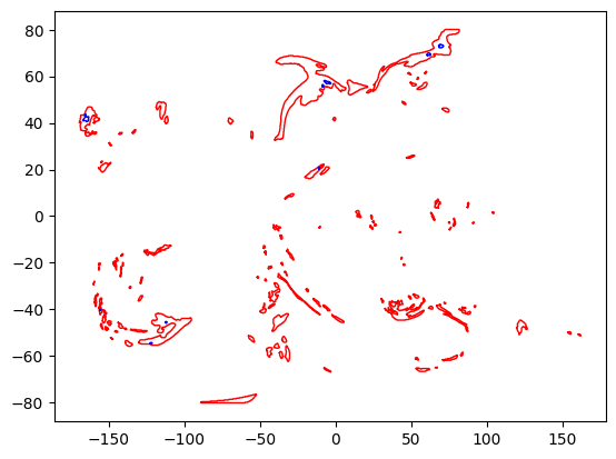
Polygon topology

GeoJSON polygons have both interior and exterior boundaries. Below use red for exterior boundaries and blue for interior boundaries.

for poly in multipoly.geoms:
    plt.plot(*poly.exterior.xy, color="red", lw=1)
    for interior in poly.interiors:
        plt.plot(*interior.xy, color="blue", lw=1)

# Print some statistics on the polygons
n_exterior_rings = len(multipoly.geoms)
n_interior_rings = sum(len(p.interiors) for p in multipoly.geoms)
n_exterior_vertices = sum(len(p.exterior.coords) for p in multipoly.geoms)
n_interior_vertices = sum(len(i.coords) for p in multipoly.geoms for i in p.interiors)
area = multipoly.area

print(f"Number of exterior rings: {n_exterior_rings}")
print(f"Number of interior rings: {n_interior_rings}")
print(f"Number of exterior vertices: {n_exterior_vertices}")
print(f"Number of interior vertices: {n_interior_vertices}")
print(f"Total area: {area}")  # units are in the image of the Plate carree projection

Number of exterior rings: 243
Number of interior rings: 68
Number of exterior vertices: 12956
Number of interior vertices: 824
Total area: 5272.312050000002

# Formalize some of cells above into functions for later use
def get_shapely(**kwargs):
    params = {
        "time": "2023-02-10",
        "format": "geojson",
        "flight_level": 360,
    }
    params.update(kwargs)

    r = requests.get(f"{URL}/v0/grid/issr", params=params, headers=headers)
    r.raise_for_status()

    geojson = r.json()
    (feature,) = geojson["features"]

    for coords in feature["geometry"]["coordinates"]:
        for poly in coords:
            for point in poly:
                del point[2]

    return shapely.from_geojson(json.dumps(feature))


def polygon_metrics(multipoly):
    n_exterior_rings = len(multipoly.geoms)
    n_interior_rings = sum(len(p.interiors) for p in multipoly.geoms)
    n_exterior_vertices = sum(len(p.exterior.coords) for p in multipoly.geoms)
    n_interior_vertices = sum(len(i.coords) for p in multipoly.geoms for i in p.interiors)
    area = multipoly.area
    return {
        "n_exterior_rings": n_exterior_rings,
        "n_interior_rings": n_interior_rings,
        "n_exterior_vertices": n_exterior_vertices,
        "n_interior_vertices": n_interior_vertices,
        "area": area,
    }

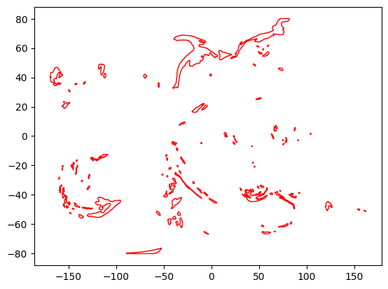
Interior polygons

Set the query parameter interiors=false to only return exterior polygons.

As seen in the polygon_metrics output and in the plot, the exterior polygons remain the same as before, but the interior polygons are removed.

multipoly = get_shapely(interiors=False)

print(polygon_metrics(multipoly))

for poly in multipoly.geoms:
    plt.plot(*poly.exterior.xy, color="red", lw=1)
    assert len(poly.interiors) == 0

{'n_exterior_rings': 243, 'n_interior_rings': 0, 'n_exterior_vertices': 12956, 'n_interior_vertices': 0, 'area': 5391.80365}

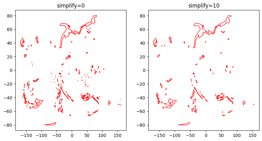
The simplify query parameter

Use the simplify query parameter to customize the extent to which polygon boundaries are simplified. This parameter is an integer between 0 and 10, inclusive. A value of 0 means no simplification. A value of 10 simplifies aggressively (thereby introducing some error). The default value is 3. A higher value also drops more small polygons.

multipoly_list = [get_shapely(interiors=False, simplify=s) for s in range(0, 11)]

# Plot the least and most aggressively simplified polygons side by side
fig, (ax1, ax2) = plt.subplots(1, 2, figsize=(10, 5))

ax1.set_title("simplify=0")
multipoly = multipoly_list[0]
for poly in multipoly.geoms:
    ax1.plot(*poly.exterior.xy, color="red", lw=1)

ax2.set_title("simplify=10")
multipoly = multipoly_list[-1]
for poly in multipoly.geoms:
    ax2.plot(*poly.exterior.xy, color="red", lw=1)

Metrics

Make a table showing how the number of polygons and vertices changes with different values of simplify.

df = pd.DataFrame([polygon_metrics(m) for m in multipoly_list])
df = df.rename_axis("simplify")
df

	n_exterior_rings	n_interior_rings	n_exterior_vertices	n_interior_vertices	area
simplify
0	308	0	18215	0	5428.75570
1	266	0	17971	0	5426.39900
2	257	0	14004	0	5406.37095
3	243	0	12956	0	5391.80365
4	238	0	10282	0	5385.11330
5	233	0	7126	0	5379.95495
6	226	0	5364	0	5374.52980
7	210	0	4328	0	5349.90020
8	204	0	3633	0	5334.65810
9	196	0	3185	0	5317.85205
10	186	0	2155	0	5206.62255

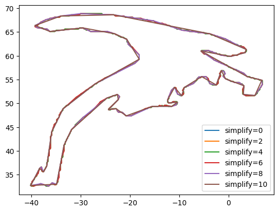
Visualize

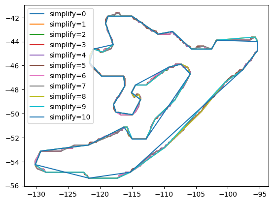
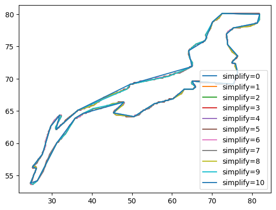
Visualize how a few of the larger polygons vary with simplify.

p0 = shapely.Point(-17, 50)

fig, ax = plt.subplots()
for i, multipoly in enumerate(multipoly_list[::2]):
    for p in multipoly.geoms:
        if p.contains(p0):
            ax.plot(*p.exterior.xy, label=f"simplify={i*2}")

ax.legend();

p0 = shapely.Point(-120, -54)

fig, ax = plt.subplots()
for i, multipoly in enumerate(multipoly_list[::2]):
    for p in multipoly.geoms:
        if p.contains(p0):
            ax.plot(*p.exterior.xy, label=f"simplify={i*2}")

ax.legend();

p0 = shapely.Point(55, 67)

fig, ax = plt.subplots()
for i, multipoly in enumerate(multipoly_list[::2]):
    for p in multipoly.geoms:
        if p.contains(p0):
            ax.plot(*p.exterior.xy, label=f"simplify={i*2}")

ax.legend();

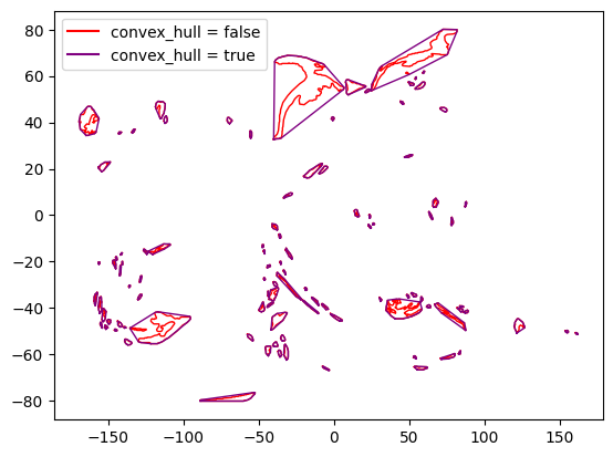
Convex hulls

Use the boolean convex_hull query parameter to simplify polygons by computing their convex hulls. When this parameter is enabled, the interiors parameter is automatically set to false.

This purpose of this parameter is to:

• Further reduce the complexity of the polygon geometry.

• Fill in “fjords” and other gaps in the polygon geometry. If polygons are regions to be avoided, points outside of a polygon but inside its convex hull may still be inaccessible for trajectory planning. By explicitly taking a convex hull, the flight planner may have an easier time creating optimal trajectories.

As seen in the table below, the number of polygons (n_exterior_rings) and the number of vertices are reduced when using the convex_hull parameter. On the other hand, the total footprint of the polygons is increased (as measured by the area metric).

multipoly_list_ch = [get_shapely(convex_hull=True, simplify=s) for s in range(0, 11)]

df1 = (
    df.drop(columns=["n_interior_rings", "n_interior_vertices"])
    .assign(convex_hull=False)
    .rename_axis("simplify", axis=0)
    .set_index("convex_hull", append=True)
)

df2 = pd.DataFrame([polygon_metrics(m) for m in multipoly_list_ch])
df2 = (
    df2.drop(columns=["n_interior_rings", "n_interior_vertices"])
    .assign(convex_hull=True)
    .rename_axis("simplify", axis=0)
    .set_index("convex_hull", append=True)
)

df = pd.concat([df1, df2], axis=0)
df.sort_index()

		n_exterior_rings	n_exterior_vertices	area
simplify	convex_hull
0	False	308	18215	5428.75570
	True	204	2891	11404.67800
1	False	266	17971	5426.39900
	True	181	2675	11401.79705
2	False	257	14004	5406.37095
	True	174	2388	11395.14875
3	False	243	12956	5391.80365
	True	168	2071	11383.98305
4	False	238	10282	5385.11330
	True	166	1836	11367.97765
5	False	233	7126	5379.95495
	True	162	1566	11337.67915
6	False	226	5364	5374.52980
	True	158	1413	11292.63095
7	False	210	4328	5349.90020
	True	147	1226	11256.84365
8	False	204	3633	5334.65810
	True	143	1097	11202.22925
9	False	196	3185	5317.85205
	True	137	1007	11158.91640
10	False	186	2155	5206.62255
	True	129	805	10982.87520

fig, ax = plt.subplots()

for poly in multipoly_list[0].geoms:
    ax.plot(*poly.exterior.xy, color="red", lw=1)

for poly in multipoly_list_ch[0].geoms:
    ax.plot(*poly.exterior.xy, color="purple", lw=1)

red_line = mlines.Line2D([], [], color="red", label="convex_hull = false")
purple_line = mlines.Line2D([], [], color="purple", label="convex_hull = true")
ax.legend(handles=[red_line, purple_line]);

Contrail forecast polygons (/v1)

Contrail forecast data served from the /v1/ API endpoints have pre-selected parameters for polygon generation.

Under the hood, forecast polygon regions are generated with the pycontrails MetDataArray.to_polygon_feature method.

For input forecast_data DataArray and threshold value, polygons are generated with the parameters:

MetDataArray(forecast_data).to_polygon_feature(**{
    iso_value=threshold,
    fill_value=0.0,
    min_area=1.0,  # corresponds to "simplify=10" query parameter above
    epsilon=0.5,   # corresponds to "simplify=10" query parameter above
    precision=2,   # for computational efficiency
    interiors=False,
    convex_hull=False,
    include_altitude=True,
    lower_bound=True
})

See Contrail Forecast /v1 notebook for details on accessing forecast polygons.