GOES Contrail Detections
This notebook demonstrates basic usage of the GOES contrail detections endpoint.
Contrail detections provided by this endpoint are generated using GOES-East Full Disk imagery and a vision-transformer-based image segmentation model from the winning solution to a Kaggle competition run by Google research.
Detections are provided at multiple data processing levels:
Level 1 (L1): Raw detection model output
Level 2 (L2): Detected contrail line segments
Detections are available in near-real-time starting at the beginning of 2024, with some minor gaps due to missing GOES imagery.
The Contrails.org API provides a Level 4 (L4) contrail attributions endpoint that is a reformatted pass-through of the Google Contrails Watch attributions product.
This notebook provides examples of using the L1 and L2 products which are generated and served by Contrails.org.
[1]:
import os

import cartopy.crs as ccrs
import matplotlib.pyplot as plt
import numpy as np
import requests
import shapely
import shapely.plotting
import xarray as xr

from pathlib import Path
from pycontrails.datalib import goes
from pycontrails.utils import temp
[2]:
# Define credentials
URL = "https://api.contrails.org"
api_key = os.environ["CONTRAILS_API_KEY"]
headers = {"x-api-key": api_key}
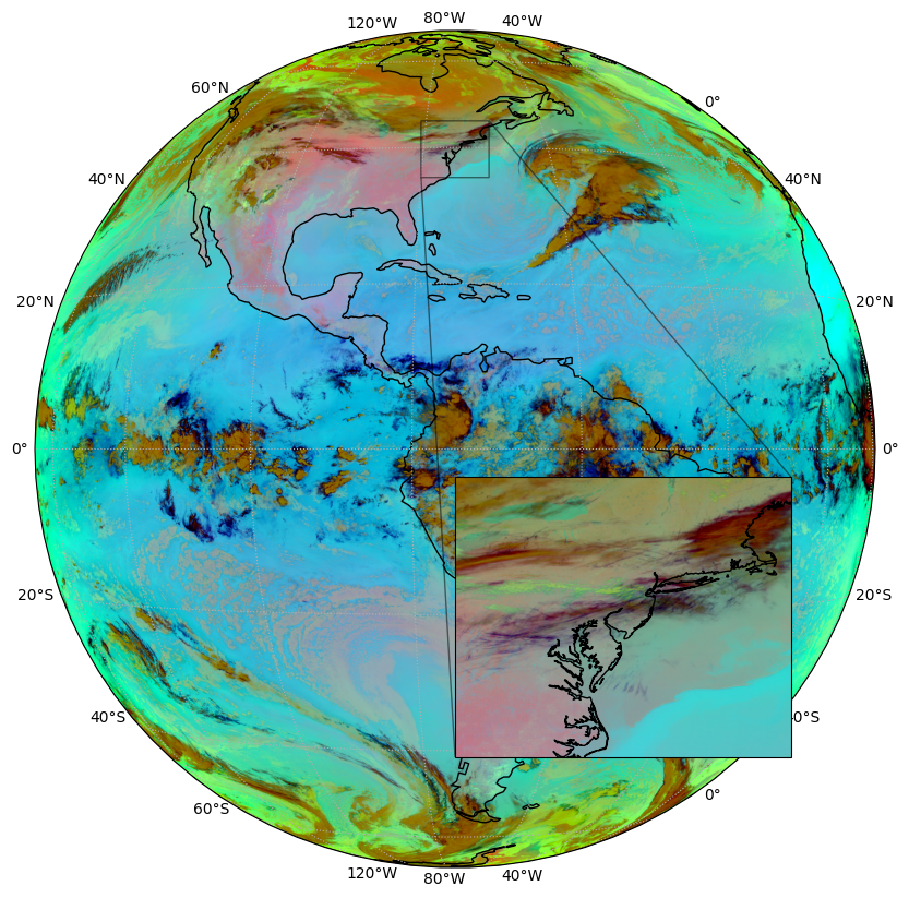
GOES-East imagery
L1 and L2 detections are both provided in the same coordinate reference system (CRS) as Full Disk GOES-East imagery. The pycontrails GOES datalib provides an easy way to retrieve GOES-East imagery and its associated CRS.
Here, we retrieve and plot imagery from the three infrared channels of the GOES Advanced Baseline Imager (ABI) used by the contrail detection model, and include an inset with details of a region that contains contrails. The color scheme shown is the so-called Ash RGB, with thin high altitude ice clouds shown in dark blue to black.
[3]:
time = "2025-03-12T12:00:00"
[4]:
handler = goes.GOES(region="full")
goes_da = handler.get(time)
rgb, crs, extent = goes.extract_goes_visualization(goes_da)
[5]:
fig = plt.figure(figsize=(10, 10))
ax = plt.subplot(111, projection=crs)
ax.imshow(rgb, extent=extent, transform=crs)
ax.coastlines()
ax.gridlines(draw_labels=True, linestyle=":")

zoom = (-80, -70, 35, 45)
inset = ax.inset_axes(bounds=(0.5, 0.1, 0.4, 0.4), projection=crs)
inset.imshow(rgb, extent=extent, transform=crs)
inset.set_extent(zoom, crs=ccrs.PlateCarree())
inset.coastlines()
indicator = ax.indicate_inset_zoom(inset, edgecolor="black")
indicator.connectors[0].set_visible(True)  # lower left
indicator.connectors[1].set_visible(False)  # upper left
indicator.connectors[2].set_visible(False)  # lower right
indicator.connectors[3].set_visible(True)  # upper right
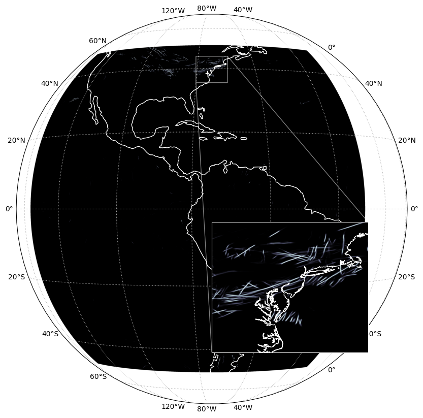
Raw detection model output (L1)
The contrail detection model computes a “confidence” that each pixel in the GOES image contains a contrail. Per-pixel confidences are computed for all pixels from 135°W to 30°W and 50°S to 50°N and can be accessed directly using the L1 GOES endpoint. The L1 endpoint returns a netCDF file that can be saved to disk and read using xarray.
Per-pixel confidences can be loosely interpreted as probabilities, but they are neither carefully calibrated nor guaranteed to be between 0 and 1.
Initial requests to this endpoint trigger a server-side job that assembles Full Disk detection masks from multiple components. This can result in fairly long request latencies (~1 minute), so we recommend submitting multiple requests asynchronously. Subsequent requests access cached Full Disk detections and have much lower latency.
[ ]:
params = {"time": time}

r = requests.get(
    f"{URL}/v1/observations/contrails-org/goes/L1/detections", params=params, headers=headers
)
print(f"HTTP Response Code: {r.status_code} {r.reason}")
HTTP Response Code: 200 OK
[7]:
with temp.temp_file() as tmp:
    with open(tmp, "wb") as f:
        f.write(r.content)
    detections_da = xr.load_dataarray(tmp)
[8]:
fig = plt.figure(figsize=(10, 10))
ax = plt.subplot(111, projection=crs)
ax.imshow(detections_da.values, extent=extent, transform=crs, cmap="bone", vmin=0, vmax=1)
ax.coastlines(color="white")
ax.gridlines(draw_labels=True, linestyle=":")

zoom = (-80, -70, 35, 45)
inset = ax.inset_axes(bounds=(0.5, 0.1, 0.4, 0.4), projection=crs)
inset.imshow(detections_da.values, extent=extent, transform=crs, cmap="bone", vmin=0, vmax=1)
inset.set_extent(zoom, crs=ccrs.PlateCarree())
inset.coastlines(color="white")
indicator = ax.indicate_inset_zoom(inset, edgecolor="white")
indicator.connectors[0].set_visible(True)  # lower left
indicator.connectors[1].set_visible(False)  # upper left
indicator.connectors[2].set_visible(False)  # lower right
indicator.connectors[3].set_visible(True)  # upper right
for spine in inset.spines.values():
    spine.set_color("white")
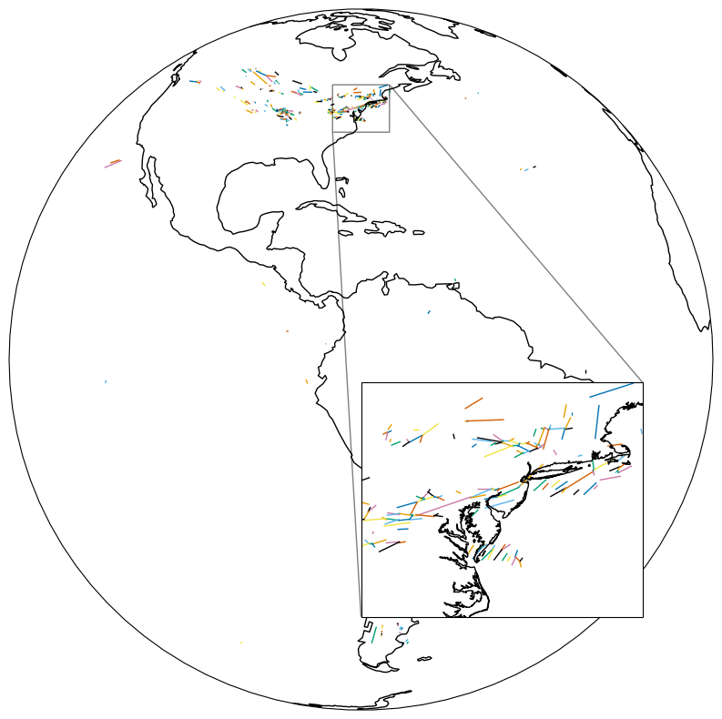
Contrails segments (L2)
Contrail segmentation takes contrail detection masks (L1) and breaks them down into individual contrail objects (L2). These objects are represented as LineStrings, which can be accessed directly using the L2 GOES endpoint (geostationary coordinates).
The segmentation comprises multiple steps:
Detection mask thresholding (0.3 used for L2 endpoint)
Connected component analysis (region proposal)
Skeletonization and branch analysis (for overlapping/crossing contrails)
The segmentation produces contrail objects of three types (see plot below):
Type N: no connections to other objects \(\rightarrow\) isolated linear contrail
Type I: one connection to another object \(\rightarrow\) one end of an overlapping contrail
Type II: two connections to another objects \(\rightarrow\) central part of an overlapping contrail
[ ]:
# Extract segments for the same time
params = {"time": time}

r = requests.get(
    f"{URL}/v1/observations/contrails-org/goes/L2/segments", params=params, headers=headers
)
print(f"HTTP Response Code: {r.status_code} {r.reason}")
HTTP Response Code: 200 OK
[10]:
# Convert WKT geometries to Shapely objects
segments = [shapely.from_wkt(segment["geometry"]) for segment in r.json()]
[11]:
# Plot segments in geostationary coordinates
fig = plt.figure(figsize=(10, 10))
ax = plt.subplot(111, projection=crs)
ax.coastlines()
ax.set_global()

zoom = (-80, -70, 35, 45)
inset = ax.inset_axes(bounds=(0.5, 0.1, 0.4, 0.4), projection=crs)
inset.set_extent(zoom, crs=ccrs.PlateCarree())
inset.coastlines()
indicator = ax.indicate_inset_zoom(inset, edgecolor="black")
indicator.connectors[0].set_visible(True)  # lower left
indicator.connectors[1].set_visible(False)  # upper left
indicator.connectors[2].set_visible(False)  # lower right
indicator.connectors[3].set_visible(True)  # upper right

segment_colors = [
    "#000000",
    "#E69F00",
    "#56B4E9",
    "#009E73",
    "#F0E442",
    "#0072B2",
    "#D55E00",
    "#CC79A7",
]
for axis in (ax, inset):
    for s_idx, segment in enumerate(segments):
        shapely.plotting.plot_line(
            segment,
            ax=axis,
            add_points=False,
            linewidth=1,
            color=segment_colors[s_idx % len(segment_colors)],
            transform=crs,
        )
[12]:
# Convert a single line segment to lat-lon
"""
NOTE: this value is not corrected for satellite perspective,
but it gives a rough idea of the location of the segment endpoints.

In order to perform flight matching, parallax correction must be applied.
"""
segment = segments[0]
coords = list(segment.coords)
x, y = zip(*coords)
segment_latlon = ccrs.PlateCarree().transform_points(crs, np.array(x), np.array(y))
lon, lat = segment_latlon[:, :2].T

print("Segment Endpoint Coordinates:")
for lon_i, lat_i in zip(lon, lat):
    print(f"Longitude: {lon_i:.2f}, Latitude: {lat_i:.2f}")
Segment Endpoint Coordinates:
Longitude: -100.38, Latitude: 49.90
Longitude: -100.19, Latitude: 49.82
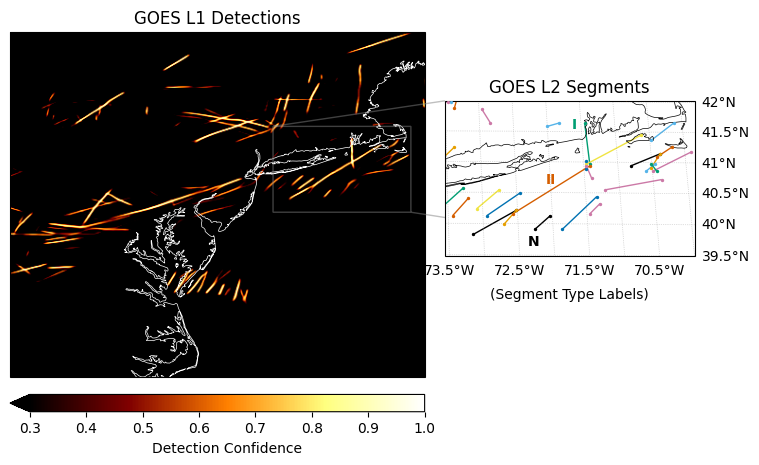
[13]:
# Plotting Detections and Segments Together
fig = plt.figure(figsize=(10, 6))
plt.subplots_adjust(left=0.1, right=0.95, top=0.9, bottom=0.1, wspace=0.05)
ax1 = plt.subplot(121, projection=crs)
ax1.set_title("GOES L1 Detections", fontsize=12)
ax1.coastlines(color="w", linewidth=0.5)
ax1.set_extent(zoom, crs=ccrs.PlateCarree())

# Plot detection mask with threshold used for L2 segment generation
confidence_threshold = 0.3
conf = ax1.imshow(
    detections_da.values,
    extent=extent,
    transform=crs,
    cmap="afmhot",
    vmin=confidence_threshold,
    vmax=1,
)
ax_cbar = ax1.inset_axes([0.0, -0.1, 1.0, 0.05])
plt.colorbar(
    conf,
    cax=ax_cbar,
    orientation="horizontal",
    pad=0.05,
    label="Detection Confidence",
    extend="min",
)

# Plot L2 segments in separate inset axes
zoom_seg1 = (-73.5, -70, 39.5, 42)
ax_seg1 = ax1.inset_axes([0.85, 0.35, 1.0, 0.45], projection=crs)
ax_seg1.set_title("GOES L2 Segments", fontsize=12)
ax_seg1.set_extent(zoom_seg1, crs=ccrs.PlateCarree())
ax_seg1.coastlines(linewidth=0.5)
gl1 = ax_seg1.gridlines(draw_labels=True, linewidth=0.5, color="gray", alpha=0.5, linestyle=":")
gl1.left_labels = False
gl1.top_labels = False
indicator1 = ax1.indicate_inset_zoom(ax_seg1, edgecolor="gray", linewidth=1.0)

for s_idx, segment in enumerate(segments):
    # Plot the line
    seg_color = segment_colors[s_idx % len(segment_colors)]
    shapely.plotting.plot_line(
        segment,
        ax=ax_seg1,
        add_points=False,
        linewidth=1,
        color=seg_color,
        transform=crs,
    )
    # Plot points separately with smaller size
    coords = list(segment.coords)
    x, y = zip(*coords)
    ax_seg1.scatter(x, y, s=2, color=seg_color, transform=crs, zorder=5)

# Labels of Type N, I, II segments
labels = ["N", "I", "II"]
lons = [-72.3, -71.6, -72.0]
lats = [39.6, 41.5, 40.6]
colors = [segment_colors[0], segment_colors[3], segment_colors[-2]]
for label, lon, lat, color in zip(labels, lons, lats, colors):
    ax_seg1.text(
        lon,
        lat,
        label,
        transform=ccrs.PlateCarree(),
        ha="center",
        va="bottom",
        fontsize=10,
        fontweight="bold",
        color=color,
        label=f"Type {label} Segment",
    )
_ = ax_seg1.text(
    0.5,
    -0.2,
    "(Segment Type Labels)",
    transform=ax_seg1.transAxes,
    ha="center",
    va="top",
)